Our main focus recently has been on the game we are developing using the Earthsim engine, but there are a few features coming up that warrant us making a small update release.
Here is a little preview of the updates for the next 0.4 alpha release.
Using the importer
We have been looking at improving the import and export features.
One of the nice things to do is to import height maps that have been generated in other tools and then add thin layers of sand, gravel or earth over them and let earthsim move those materials.
Here are some examples of earth & sand deposition over imported height maps
We are looking at what other features we could add. Being able to export the type map into the height map png file is also an option using the 8bit greyscale + 8bit alpha format in the png spec. But obviously this limits the height resolution to 256 levels. This would be an ideal format for user created brushes or bump map textures to be used in a game.
Dynamic paint and saveing layermaps
Everyone wants to be able to paint directly onto earthsims layermap. Its much more dynamic and fun. We have implemented an experimental version of this but there are a few technical challenges we need to finish off before we can deliver the feature.
Earthsim currently records all its user land edits into the layer map so any part of the world can easily be recreated and changed. As soon as you start painting on the landscape we need to start recording ‘strokes’ and this requires an extension and update to the current ‘sim file format. We also need to add support to be able to edit the strokes from the layer editor.
The biggest feature here though is the ability to save and load eroded layermaps directly in a binary format. The main challenge here is that layermaps can get very large. But this is very much needed for the game, to so it has to come soon, it also makes the features for ‘paint’ make sense for an update.
Layermap save and load. (save partially eroded ‘live’ layer maps)
Non destructive support of user imported data in the layer editor.
Our engine is arriving at a point where there is enough in place for us to have confidence we can achieve our goals with the overall design direction.
The engine can simulate and visualize water, earth, sand movement and rock erosion on tiles of 2048 square, up to 32k square depending on the power of the PC being used. Along with a biosphere of over 1million trees and plants growing on it. The baseline resolution of a world is 2048×2048.
Our initial technology goals are achieved and we know we can do what we want to do on a PC. Over time we can work to push these out further.
We will now work toward polishing up some of these features to get them out into a first engine release.
As the engine is coming together, we are at an important point on the game design cycle. Which way we decide to go will determine the back story that the game world fits into.
Earthsim TGM 1.0 worlds are square 10x10km tiles. We need to decide what we are going to do at the end of the world, the edges of the tile. There are two options outlined below:
Skybox
This option does not let the camera come outside of the main tile, and uses a skybox to surround the world with an image to create the feeling of being inside a greater reality.
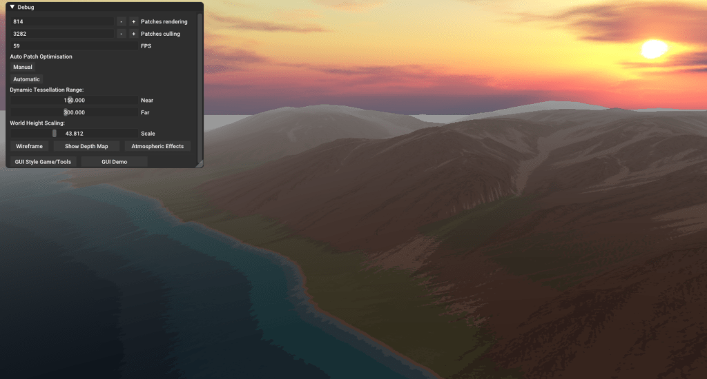
This is very common in games as it can look fantastic when done well. It is sort of cheating like the Truman show. Limits on camera motion and position impact on the type of gameplay you can access on the world.
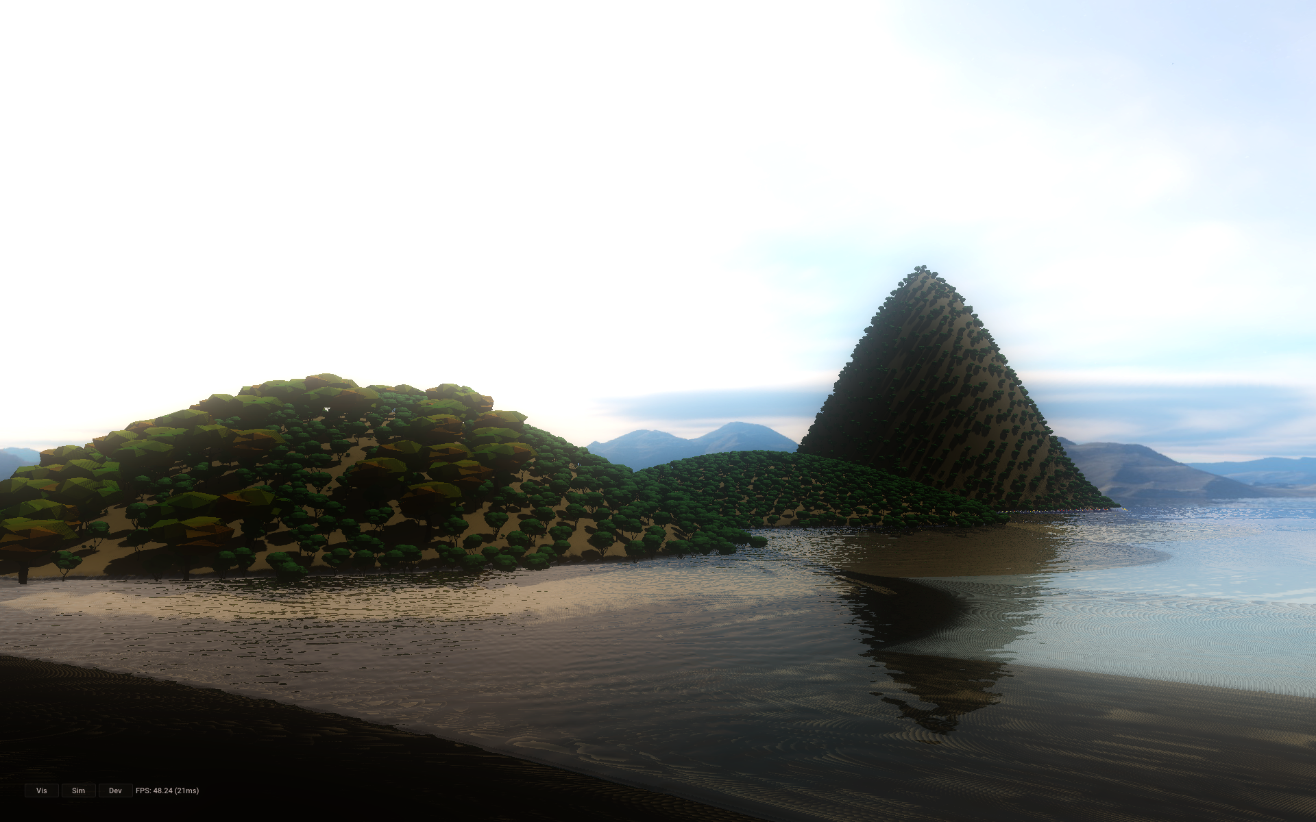
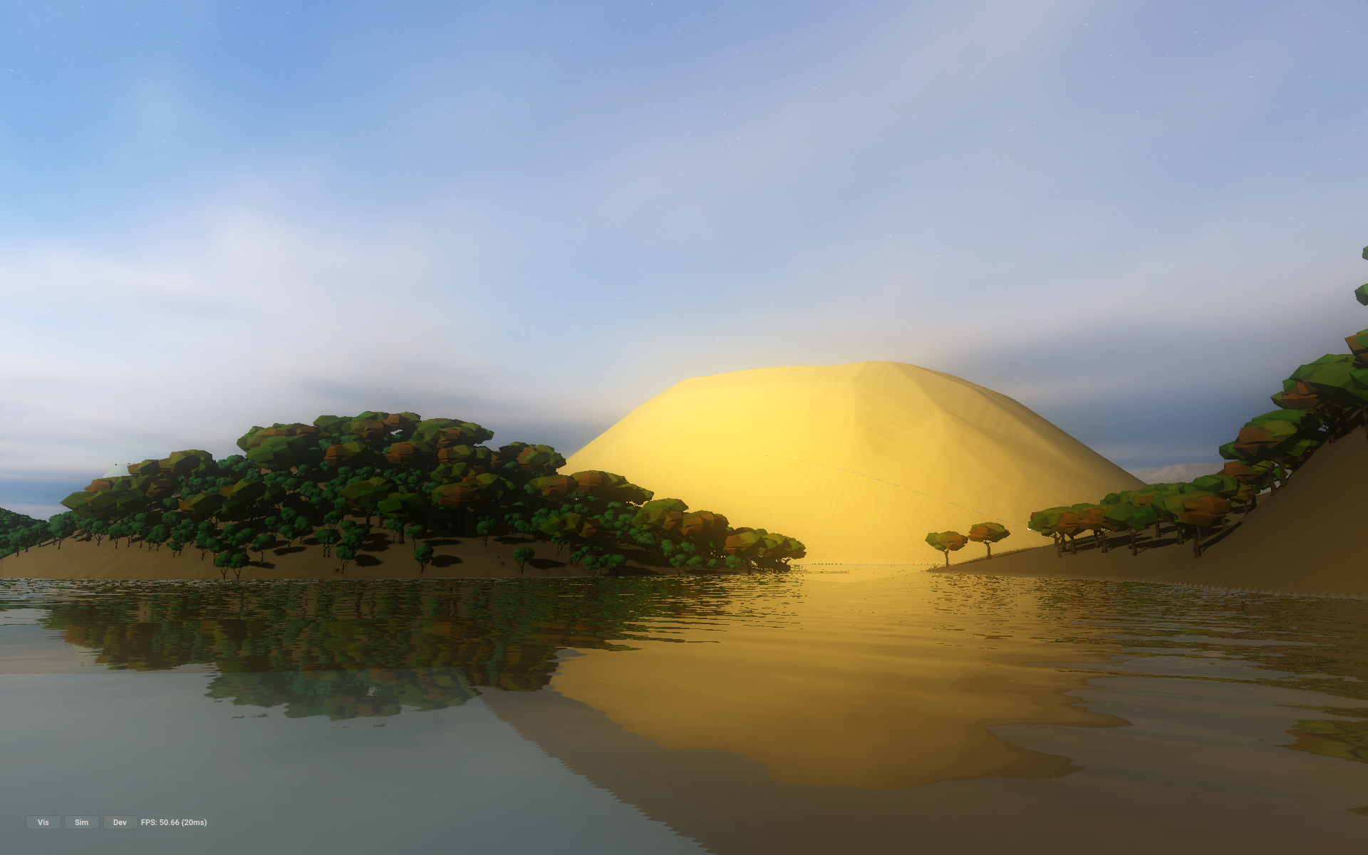
The current demo is using a skybox, all the three images are taken out of the latest demo build of Earthsim TGM using a standard skybox for the background and clouds. This does look really nice and feels very convincing as an immersive world. But if you move the camera high up or to beyond the edge of the tile, that illusion quickly breaks.
Aquarium
The simulation world is limited, this is the reality of any game other than infinitely procedurally generated worlds. Instead of trying to hide this limit, show the world tile as some sort of ‘aquarium’. This requires us to create a cross section rendering system so ‘cutaways’ can been seen at the sides of the aquarium, to show layer cross section of the land surface and water. The images below from 3d map generator are good examples of this style.
TGM is more a god mode game than an immersive world game, so we are beginning to lean toward the aquarium style. We will be adding rendering features to create the cutaway cross section and and will be looking to create the game story around this style.
Other News: bgfx
We are working on moving our rendering back end over to the bgfx cross platform rendering library. This gives us a quick path to running many 3D hardware configurations and API’s. Progress so far is good and if all continues to go well, the next demo release in May will be running on it.
You can follow us on twitter. Or If you have feedback or ideas on these directions, feel free to jump into our discord server and let us know: https://discord.gg/h8aDJthTk5.
Water forms a big part of the earthsim3 engine. There are two major challenging components to this.
Simulating a large amount of interconnected bodies of water in real time
Rendering a large scale landscape that has dynamic simulated water on it.
Water Simulation
Like pretty much everything in the world of computers, the fundamental limit to what you can do is down to memory. How much of it you can access and how fast you can get to it.
Water simulation is no different. The maths for how to do it is pretty straight forward, the challenges come in making a fast usable implementation that can work for a game.
Realtime water simulations work very well on the GPU, the GPU is ideally suited for massive batch processing of the water data. But we want the Earthsim landscape to be big, 8k, 16k and even 32k landscapes should be possible for people that have a machine setup for it.
For example, a 16k x 16k tile of landscape gives you 268 Mega cells (each cell is one pixel of land data). If the memory use per cell of landscape (water simulation variables + land type layers) is say 64 bytes. A 16k landscape takes over 17 Gigabytes of memory!
It is not possible to fit this scale of landscape on the GPU and leave a decent amount of space for both the frame buffer and atmosphere voxel buffer.
It becomes clear from memory alone that land and water simulation have to go on the CPU. This leaves the GPU to do rendering, and atmospheric simulation. That’s plenty to keep a GPU busy, especially if we ray trace the dynamic atmosphere as we hope to do.
Luckily there are two features of modern CPU’s that make this doable.
Multi core is happening in a big way, especially with the latest AMD processors.
SIMD code on the CPU is beginning to bring you into the ballpark of GPU speed.
AMD has the edge right now on core counts, but Intel has 16 way SIMD with AVX512. This should give it a 2x advantage over a similar AMD core that only has AVX2.
Its going to be fascinating to build a simulation benchmark out of this and try out some of the latest CPU’s.
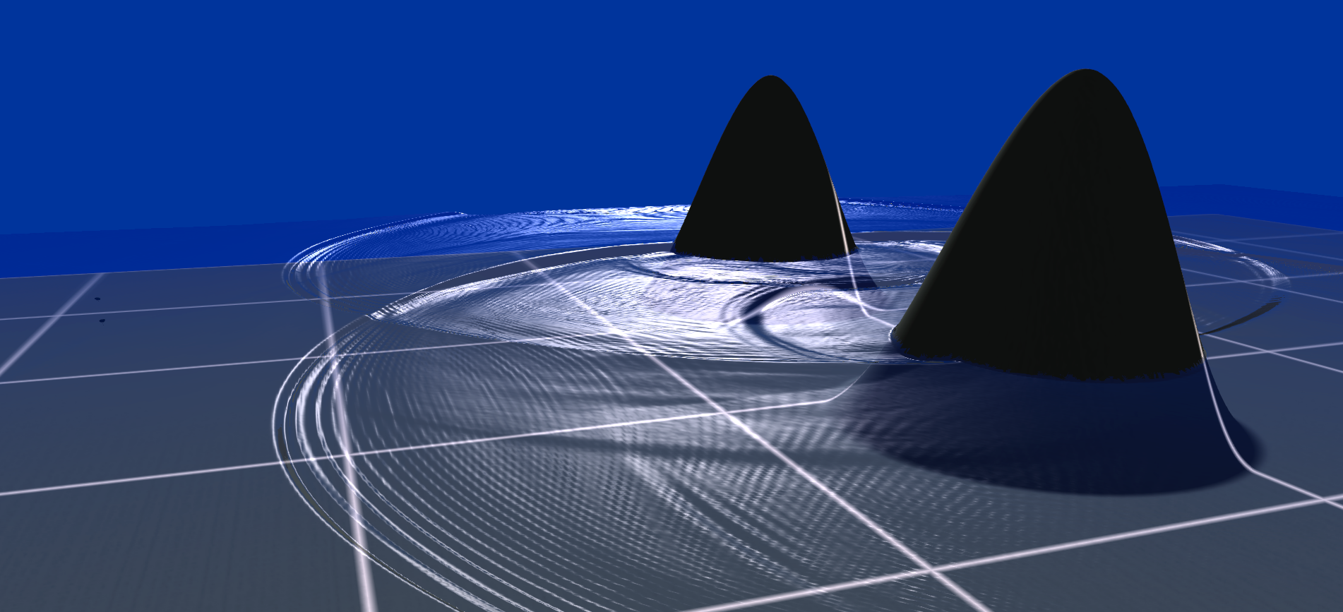
The landscape is divided up into tiles, each of which can run on an independent CPU core. This video shows the water running in separate tiles (looking like aquariums in the video) This was the first step that we used to prove out if the performance of a CPU SIMD implementation was good enough. It was.
The next step is to getting the code to run on multiple cores and hand the data between the cores at the edges in a fast enough way. Its coming along well but still has some bugs and work todo before its done.
Early debugging on the water tiles
More bugfixes in water simulation and the tiles are joining up well. But there are still some high frequency artifacts coming into the simulation. This is now running an 8×8 tile grid (256 per tile). This is still all one one core, running the optimized version of the code, but has dropped to 30Hz.
Water Rendering
Once again, the challenge in rendering the water is all about memory. For our 16k x 16k example tile of 268 Mega cells, if the water heights alone were 2 bytes, that’s a half gigabyte to get from the CPU to the GPU every frame.
Add to this that the land in earthsim3 is also alive with:
real-time erosion
sand/earth/gravel settling
lava moving
That adds another 3 bytes of data (2 for land height and 1 for type). To give over a gigabyte of data uploading to the GPU every frame. That’s too much to run at 60Hz.
This 1gig+ upload is then turned into a pyramid of LOD’s dynamically by the GPU to render the landscape. It is worth adding view frustum culling to the up-loader so we only load the LOD’s that are visible to the GPU, but that means calculating the LOD’s on the CPU. This should be relatively cost free to combine into the water and tallus engines.
Additionally the land updates don’t need to run quite as fast as the water. Water looks great at full framerate 60 or 120 Hz. But land updates can happen 2x or 3x slower and its hardly noticeable as sand movement, land settling and erosion all are much less dynamic effects.
After all this is working, the next step will be to look into a few simple real-time compression schemes for the data. Even a 2x reduction in data would make a large difference. Realtime DXT compression should do the trick and bring in another 2-4x on size.
Finally because we have a map of what each type of surface value is, we can make an intelligent landscape extrapolate on the GPU to give us 2-4x extra detail on there for rendering. The extrapolator is well understood technology so will come later once the parts we are less sure about are finished off.
For the new engine. I have been designing a genome model for the biosphere. This is the set of genes that describe any plant that can grow in Earthsim’s biosphere. Each gene has a specific function in the plant.
To do this well I needed to have a good idea of the model that the trees and plants would be growing inside.
Once you have a good understanding of the model. You can know what genes to put in a plant description so it can optimise itself for growing in the environment.
Below is the model for how water can move around on the land.
The land simulator manages this water for us, so we will know exactly how much water we have in any of these components.
This water availability is used by the Biosphere simulation to know where and how trees can grow.
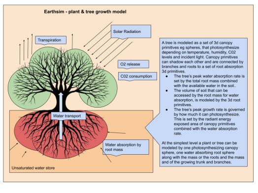
Here is the summary design of the plant/tree model that works with the above.
A few interesting points to note about this model. (When I mention a tree it also applies to any plant)
Trees can self shadow, so sections of a tree can be less efficient and can die away. So a tree can grow and change shape over time.
Trees and plants have a few interesting dilemmas they need to solve with their different genetic makeups.
When they want to photosynthesize, they have to open their pores. But when they open their pores, if the air is hot, the can loose much more water to the air than they would want. Trees that can manage when they open or close their pores can survive better in arid climates.
Tree’s that have leaves that can be damaged by the cold have to decide when to drop and when to grow their leaves.
Tree’s that have seed/fruit that can be damaged by the cold. or that can require much more water and energy to grow also have to manage their timings.
Tree canopies heat up from sunlight, but you can still photo synthesize from indirect illumination. Hence different canopy and leaf configurations offer different competitive factors for optimization.
The critical thing about all this is that it lets us know how much new water vapor and C02 is added to the atmosphere by a forest. And we can model what happens to the atmosphere as we change the forest.
Here is the diagram of the top level model that these pieces fit into.
Dave and I have started working together on Earthsim.
We have started with a clean slate and are writing pretty much everything from scratch. But times have changed, there is so much open source out there that we can base many components on existing technologies. This leaves us clear to focus on just the pieces we want to specialize on.
We have already set out some of our goals for the game and what the engine needs to do:
Simulate an 10km square tile of landscape. At least 2k resolution and upto 32k x 32k resolution.
Simulate a million plants & trees for the 10km square.
Above is our first screenshot from getting the first rendering prototype drawing a test landscape. Dave is building out the DirectX parts of the engine while I work on the model for how all our plants and trees grow.
Hierarchical grids and real time data compression
The most fundamental gate on performances is the speed a processor can get to its memory. It does not matter how fast you make your processing. If the data IO takes longer than the computer speed, the IO speed is the limit of performance.
Essentially, if you want to process big things fast, you have to make the memory use smaller.
Storing vast data sets at high performance needs real-time data compression. Otherwise you can easily run out of cache, and not manage to read in your data fast enough to keep the CPU or GPU running at a speed it should be. You stall.
One way of achieving this is to use hierarchical grids running at multiple resolutions that divide a world up into successively smaller cells, each with their own sub coordinate systems.
These sub-coordinate systems let us store plant and creature positions relative to their closest grid cell. So we can often use half precision floating point and sometimes even 8 bit fixed point precision to give a 4x data improvement over normal size floating point data. And this gain translates directly to performances gains.
Here is the design I just finished for our simulation grids. This shows all the different grid resolutions we are using to model and simulate our ecosystem.
(right click to open in a new tab if you really want to see the grids)
These grids also enable the algorithms to be more easily multi threaded for many core parallel performance, as well as enabling us to precisely tune the code so that all data fits by design ideally into the first and otherwise the second level CPU cache over a complete data processing loop. This removes the requirement of the CPU to fetch new data from main memory until a given cell’s work is complete and sent back out of the cache to main memory.
We want all performance critical code to be running in this fashion so performance is gated on first or second level cache speed rather than main memory speed.